Compute-Optimal Scaling for Value-Based Deep RL August 2025
Preston Fu*, Oleh Rybkin*, Zhiyuan Zhou, Michal Nauman, Pieter Abbeel, Sergey Levine, Aviral Kumar
NeurIPS, 2025
Value-Based Deep RL Scales Predictably February 2025
Oleh Rybkin, Michal Nauman, Preston Fu, Charlie Snell, Pieter Abbeel, Sergey Levine, Aviral Kumar
ICML, 2025
ICLR Robot Learning Workshop, 2025 (oral)
In the era of large-scale AI, it is important to prototype new training methodologies at small scales before running at large scales or datasets. This workflow only works if the training outcomes are predictable — we need experimentation workflows for which results at small scale can reliably forecast behavior at large scale without running the full experiment. To build predictable workflows, the community has followed the path of estimating scaling laws: rules that fit the target performance metric as a function of resources (e.g., data, compute) available to the practitioner under the “right” design decisions for setting up training. Scaling laws can then inform practitioners how to most reliably obtain performance at scale. For example, prior work establishes that it is possible to estimate the best batch size and model width and depth from small-scale runs, and leverages this predictability to predict the best configuration for an extrapolated model size. Can we build similar workflows for reinforcement learning (RL) algorithms? In this blog post, we explore whether we can derive scaling laws for online RL algorithms.
Our blog is based on a series of two papers that challenge the conventional wisdom that value-based off-policy RL methods are fundamentally unpredictable. As we discuss below, as long as we follow careful workflows to predict hyperparameters, value-based RL is predictable. That said, establishing scaling laws for off-policy RL is substantially harder than standard LLM training: while most scaling law studies assume a fixed data distribution, RL admits a moving data distribution and accumulation of previous data (”replay buffers”).
Figure 1: We are able to estimate scaling laws for value-based RL. Data efficiency is predictable with respect to UTD and model size, unlocking compute-optimal scaling.
Part I: Challenges of estimating scaling laws for RL
Let’s start by attempting to understand the challenges we need to resolve to estimate scaling laws for RL. Scaling laws typically answer:
Given a large, unseen budget on resources (i.e., data and compute for our study), how can we achieve the best possible performance?
To make this question concrete, let’s work through the case of LLM pre-training. In LLM research, the budget corresponds to the total compute used for training, measured in FLOPs, and the performance metric is test perplexity. This budget can be further decomposed into a function of the model size, the dataset size, and hyperparameters (number of epochs and batch size):
Within this framework, researchers have arrived at conclusions on the optimal data-epoch tradeoff, the data-model tradeoff, and the critical batch size, together prescribing rules for setting hyperparameters and characterizing how performance metrics depend on available resources when hyperparameters are set accordingly. This enabled simple power laws forecasting the loss in terms of model size and dataset size. With the right batch size and epoch count, balancing between model size and dataset size laid the groundwork to train large models compute-optimally.
We follow a similar protocol for RL, though hyperparameters and performance metrics vary substantially between LLM pre-training and RL. We first describe how RL scaling laws are different, then dive into estimating them.
What makes RL scaling laws different?
Let’s now make the scaling question concrete in the context of RL. While LLM pre-training assumes access to i.i.d. high-quality training data, in RL, data is collected by the learning algorithm itself, which means that data is now a resource. Indeed RL research often optimizes for sample-efficiency, in an attempt to maximize performance given a fixed number of samples. We will denote the resource of data as . In addition, like pre-training, RL will spend FLOPs during training, which means compute spent training on the data is still a resource. While compute depends on data for any ML procedure, online RL collects data “in-the-loop” by running intermediate policies online — meaning that the process of data collection itself spends additional time or GPU/CPU computation. Therefore, it is more beneficial to consider a more holistic notion of budget that combines and : , where is a domain-specific constant.
The performance metric is an agent’s performance, i.e. the average return attained by the agent. This setup gives us our problem statement:
Given a limited budget , on a combination of compute and data, how do we achieve the best possible return ?
In practice, this problem is hard to answer directly, since reward transformations can make return unpredictable without actually changing the optimal policy at all. Therefore, we’ll consider the dual problem. Define data efficiency and compute efficiency as the amounts of data and compute needed to achieve performance , respectively. Then, the best possible that we can attain given the budget should be the one where we have used up exactly the allocated budget, i.e., . So, we can instead estimate and for multiple , then select the largest fitting within the budget . This results in a different scaling question that we will study in this line of work:
Given a performance threshold , how can we allocate our resources to minimize the budget ?
Scaling laws have been studied for on-policy algorithms, like PPO and GRPO. On-policy algorithms iteratively collect a batch of trajectories from the current policy , score those trajectories, and take a gradient step toward high-scoring trajectories (perhaps subject to constraints). At each iteration, once the update is done, the data must be thrown away, and a new batch is collected from the new policy. This highlights a data efficiency limitation: on-policy algorithms discard data, and is not optimal at minimizing budgets. Thus, we turn to off-policy RL, which can learn from data collected by policies other than . We briefly review off-policy RL.
Primer on off-policy RL
Modern off-policy RL typically trains a value function . The learned value function is agnostic to the policy used to collect state-action transitions (”behavior policy”) – instead, these transitions are sampled from a replay buffer storing all past transitions. The Q-function then aims to estimate the expected reward under the learned policy. In practice, the Q-network is trained by regressing onto a bootstrapped target, called the temporal difference (TD)-target , where comes from a stale copy of the Q-network, often called the target network. The regression loss, which is referred to as the temporal difference error (TD error) is given by:
Regressing onto TD-targets introduces complexities that we need to account for when scaling:
- The TD-targets are moving because depends on .
- Replay buffer introduces staleness because we revisit old data and train on it multiple times.
However, this second mechanism is exactly what makes TD-learning compelling in data-limited regimes like robotic learning: we can reuse expensive experience many times. Intuitively, we can scale compute for a given amount of data by just taking multiple gradient steps on each batch sampled from the replay buffer. This can be quantified by a ratio: updates-to-data ratio (UTD).
Going back, we can define the total compute utilized as follows:
This gives us multiple ways to control budget in RL: one approach is to increase the UTD ratio, training more on the same data while reducing the amount of new data collected; another is to increase model size, enabling better learning from the same data. A third approach is to use both small model size and UTD ratio, but collect more data. However, these configurations do not behave identically. For example, it is well known that increasing the UTD ratio improves performance at small values, but increasing it excessively can degrade performance, a form of “overfitting.” In repetitive, long-horizon tasks designed for scalability with horizon reduction, it was shown that scaling the model size led to plateauing performance. Likewise, while larger models can reduce the required amount of data , it is known that smaller models can reduce the required amount of compute .
Accordingly, we need to be quite careful when studying scaling laws for RL. Unlike pre-training, where models see each data point over a small number of epochs, off-policy RL repeatedly trains on the same data and is thus more prone to overfitting (see footnote). Nevertheless, the optimal budget-minimizing solution appears to require passing over the same data more than once, which raises the question of how to set hyperparameters in the presence of overfitting. Empirically, we find that choosing the correct batch size and learning rate mitigates overfitting in both cases and enables scaling to higher UTD ratios and model sizes, as we discuss next.
Part II: How do I set my hyperparameters…
A key ingredient enabling scaling laws for pre-training is the wide array of theoretical and practical results establishing the relationship between optimal batch size, learning rate, and optimizer. Put together, these trends enable hyperparameter transfer to unseen model sizes.
In our answer to this question, we unlock several surprising findings on off-policy RL training dynamics, which we later leverage to scale UTD and model size effectively.
…when I scale the UTD?
Let’s first look at the case of UTD-only scaling at a constant model size. Empirically, we find that performance is most sensitive to changes in batch size and learning rate, and we’ll focus on these hyperparameters.
Let’s first consider the effect of UTD scaling on the training data. For the purposes of this discussion, we define “overfitting” as the difference between TD errors on data sampled uniformly at random from the replay buffer and the data most recently added to the replay buffer. Intuitively, high UTD and high batch size both see a typical sample more times and overfit to those samples. This results in higher relative TD error on data recently collected by the policy . We also observe the same empirically. To counteract this effect, we decrease the batch size for higher UTD.
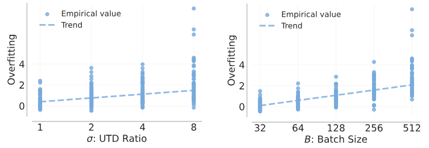
Figure 2: Overfitting increases with both UTD and batch size.
Next, let’s consider the effect of UTD scaling on Q-learning dynamics. Increasing the UTD aims to fit too well to the previous TD-target, making it more difficult to fit TD-targets later in training. Similarly, we observed that higher learning rates lead to high-magnitude updates against the target, moving the parameters to a state that would suffer from difficulty in fitting subsequent targets. Following prior work, we empirically find that one diagnosis for this plasticity loss is large parameter norm in the Q-network: increasing either UTD or learning rate corresponds to larger parameter norm. To counteract this effect, we decrease the learning rate for higher UTD.
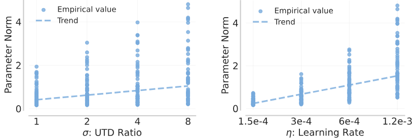
Figure 3: Parameter norm, a proxy for plasticity loss, increases with both UTD and learning rate.
The best-choice batch size and learning rate are predictable functions of the UTD ratio, and both decay as power laws.
…when I scale the model size?
Let’s now look at the case of model size scaling at a constant UTD. Generally, larger models are better performant, but it is unclear how one should set other hyperparameters when model size is increased. Model size scaling is a complementary approach to scaling compute which does not require taking multiple updates on the same data, so we’ll instead directly measure the Q-network’s generalization capabilities. To do so, we measure the TD error on both the training data and a held-out validation set of transitions drawn from a replay buffer with the same distribution.
Figure 4: Training and validation TD-errors reduce as model size increase. However, for smaller models, a larger batch size results in a higher final TD-error. This illustrates the role of batch size in modulating overfitting with TD-learning.
Unsurprisingly, increasing the batch size improves training TD-error. However, the effect on validation TD-error is more nuanced and depends on the model size. Why does this happen?
We find that small Q-nets produce TD-targets that generalize poorly, which is exacerbated by larger batch sizes. Larger Q-networks produce better TD-targets and can benefit from large batch sizes. We encourage you to check out our understanding of this phenomenon, which we coin TD-overfitting, in the deep dive below.
So, how do I set my batch size? Empirically, we observe that the best batch size increases with model size, but eventually reaches an upward asymptote. Check out our new paper for our fit equation! Empirically we do not observe a significant interaction effect between UTD and model size, i.e. our fit factorizes into a power law decay in UTD and an upward asymptote in model size.
How about other key hyperparameters? In our new paper, we additionally consider the effect of learning rate (Appendix D.2) and the target update rate (Appendix D.3). For “reasonable” selections of those hyperparameters, we found that data efficiency was most sensitive to changes in batch size. These hyperparameters still depend on the UTD ratio, but they are less sensitive to model size alone.
- TD-overfitting: Overfitting is a result of poor generalization of TD-targets from smaller models.
- With low model capacity, increasing batch size results in a higher validation TD-error; with high model capacity, increasing batch size results in a lower validation TD-error.
- The best batch size increases with model size and decreases with the UTD ratio.
Part IIIa: Budget-optimal scaling for off-policy RL
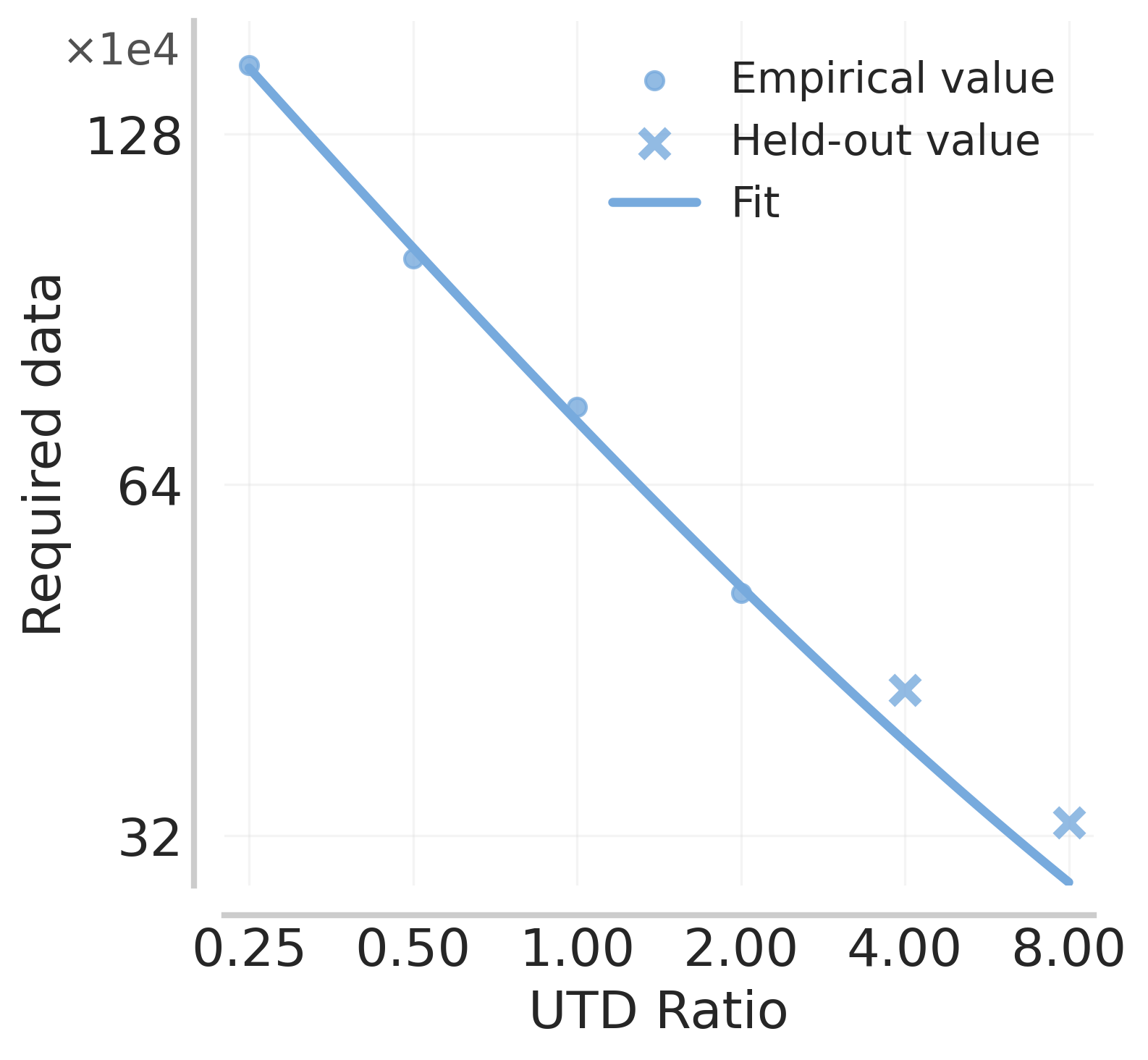
With the design of hyperparameters above, we now attempt to put together scaling laws as a function of the total budget given to us. As before, we’ll first consider UTD-only scaling at a constant model size. Armed with the best-choice batch size and learning rate, we can optimize the data efficiency. Empirically, we find that data efficiency scales as a power law with respect to UTD, across multiple domains, tasks, and algorithms!
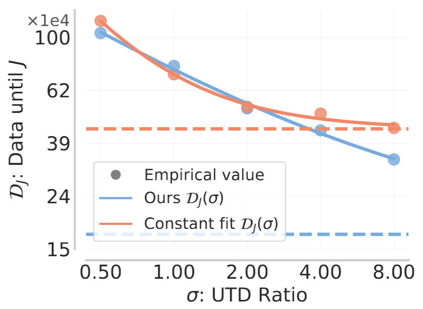
Figure 5: Data efficiency scales as a power law with respect to UTD. Leveraging the batch size and learning rate fits asymptotically outperforms a constant baseline.
Finally, we are in a position to answer our question:
Given a performance threshold , what is the minimum achievable budget , where the data efficiency and compute efficiency are the amounts of data and compute spent to achieve performance ?
We can consider the amount of compute, in FLOPs, required to achieve a given performance threshold. For each performance threshold, there is a Pareto frontier defining the tradeoff between data and compute requirements, and the UTD defines the position along this curve. Along this Pareto frontier, there is a unique budget-minimizing choice of UTD. In our paper, we showed that the budget-optimal partition between data and compute is predictable, as well as the budget-optimal UTD itself!
This tradeoff is predictable across multiple domains and algorithms. Moreover, the budget-optimal UTD extrapolates well to larger budgets! Our scaling laws let you predict the best data-compute tradeoff, parametrized by the UTD, at unseen budgets.
Figure 6: Each contour is the curve attaining the same fitted data efficiency to achieve a given target performance . The budget-optimal UTD and model size are marked with stars.
- Leveraging the best batch size and learning rate, the data efficiency decreases as a power-law in the UTD ratio.
- For each threshold, the UTD defines a Pareto frontier between data and compute requirements.
- The budget-optimal UTD is predictable, following a power law that can extrapolate to large budgets.
Part IIIb: Budget-optimal scaling for UTD and model size
Now, we’ll additionally leverage incorporate model size into our fit. To do so, we will use our knowledge of the TD-overfitting phenomenon (see deep dive), which prescribes how batch sizes must be set when model size is changed. Long story short, we find that data efficiency scales as a sum of power laws with respect to the UTD and model size. (In Section 6 of our new paper, we also run a sensitivity analysis to show the importance of using the right batch size.)
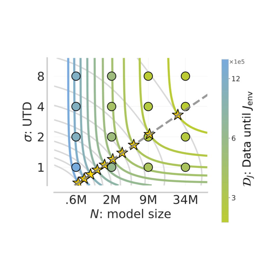
Figure 7: Each contour is the curve attaining the same fitted data efficiency to achieve a given target performance . The budget-optimal UTD and model size are marked with stars.
Conveniently, our fit equation admits a closed-form solution for budget-optimal UTD and model size, in terms of the data efficiency! We find that, within a given budget, UTD-only scaling and model-size–only scaling use 11% and 26% more data, respectively, compared to the compute-optimal setting. In the paper, we similarly show that the data–compute partition is predictable at extrapolated budgets – check it out!
- Leveraging the best batch size, data efficiency can be modeled as a sum of power laws decaying in UTD and model size.
- Our fits tell you whether it is more compute-efficient to scale your UTD or model size.
A call for scalable RL algorithms
Scaling laws provide a blueprint for building RL methods that scales. By identifying the scalable regime, we show that value-based RL admits predictable scaling once its core instabilities, which manifests as overfitting, are resolved. In pre-training, scaling laws depend on the best choice of model size, batch size, and learning rate. In value-based RL, these relationships are much trickier to uncover, due to data distribution shift and the use of target networks in practice. These training dynamics are associated with a suite of parameters including the replay buffer size, optimizer, loss function (here, a distributional RL critic), and actor update frequency. Each new axis adds to the foundation for compute-optimal training, and scaling law research can extend to new parameters and training regimes.
Ultimately, though, we must not only characterize existing methods, but also design better algorithms. We urge the field to provide systematic scalability studies:
Step 1: Characterize scaling in existing algorithms.
Step 2: Use scaling laws to select the best-performing methods.
Step 3: Design new algorithms that scale more reliably across domains and budgets.
The goal is not just to show that RL can scale, but to establish a framework where scaling laws guide the design of the next generation of scalable RL techniques. We believe this direction is key to unlocking value-based RL for larger-scale practical applications, such as LLM agents.
Deep dive: how does overfitting manifest with model size scaling?
In Figure 4, we observed that for small models, larger batch sizes worsened generalization; for large models, larger batch sizes helped. (See Appendix B of our new paper for more details on constructing the validation dataset). It’s helpful to look at these curves over the course of training, since in the practical implementation of TD-learning, value functions rarely fully fit the moving TD-targets.
Conceptual view: We argue that this deviation from classical overfitting is explained by the use of target networks in TD-learning, and coin this phenomenon TD-overfitting. Consider a smaller value function. Due to its low representational capacity, a model would entangle features used for predicting Q-values across multiple (state, action) pairs. As we scale up the batch size, this issue is exacerbated since these incorrect gradient updates become more “directed”. Fitting the Q-function, and hence the TD-targets, on some transitions comes at the expense of others.
By contrast, larger value functions produce features that can decouple its predictions across transitions, leading to improved generalization at larger batch sizes.
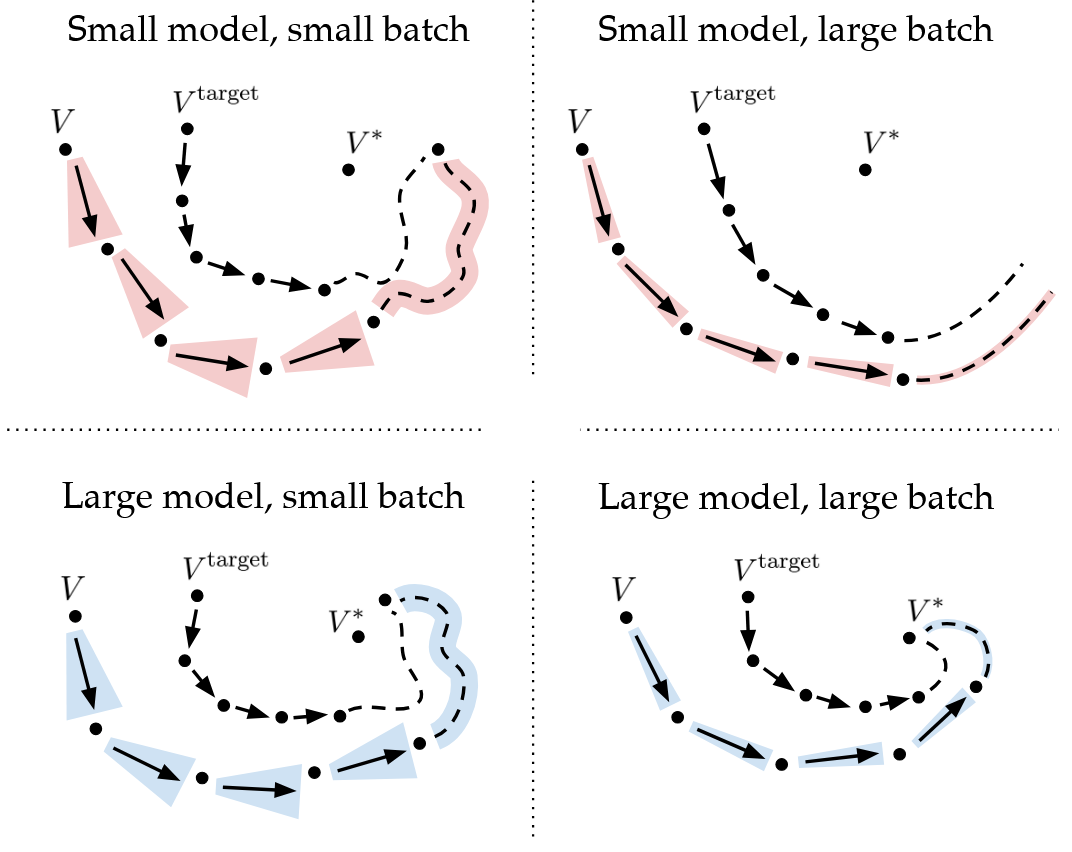
Figure 8: Small models perform better with smaller batch sizes, which result in noisy updates, due to more directed gradient updates onto low-quality TD-targets. Larger models produce higher-quality TD targets and benefit from regressing to these targets better with larger batch sizes.
Check out our new paper (Section 5.3) for an empirical analysis of this phenomenon! Or go back to the model scaling section.
Why is overfitting especially problematic in value-based RL?
Language model research has shown that training on the same data more than 4 times yields diminishing returns. For contrast, we can compute this number in off-policy RL training. In simulated robotic tasks, we typically “seed” a replay buffer with transitions, use a batch size , and train for up to transitions. By linearity of expectation, the th element in the replay buffer is expected to be sampled in
training iterations (assuming sampling with replacement; we approximate since the replay buffer is typically much larger than the batch size). For the case, we can approximate this as , i.e. the initial “seed” data is trained on around 2700 times. It is this orders-of-magnitude difference that explains the importance of studying overfitting in off-policy RL training.
Link back to our primer on off-policy RL.
Acknowledgments
We would like to thank Zhiyuan Zhou for his helpful feedback on this post. The views in this blog are our own and do not necessarily reflect those of our coauthors.
Citation
@article{fu2025scaling,
  title = {Scaling Laws for Value-Based RL},
  author = {Fu, Preston and Rybkin, Oleh and Kumar, Aviral},
  journal = {value-scaling.github.io},
  year = {2025},
  month = {September},
  url = "https://value-scaling.github.io/"
}
References
Hilton et al. Scaling laws for single-agent reinforcement learning. arXiv, 2023.
Hoffmann et al. Training compute-optimal large language models. NeurIPS, 2023.
Kaplan et al. Scaling laws for neural language models. arXiv, 2020.
Krizhevsky. One weird trick for parallelizing convolutional neural networks. arXiv, 2014.
Kumar et al. Offline Q-Learning on Diverse Multi-Task Data Both Scales And Generalizes. ICLR, 2023.
McCandlish et al. An empirical model of large-batch training. arXiv, 2018.
Muennighoff et al. Scaling data-constrained language models. NeurIPS, 2023.
Nikishin et al. The primacy bias in deep reinforcement learning. ICML, 2022.
Park. Q-learning is not yet scalable. 2025.
Schulman et al. Proximal Policy Optimization Algorithms. arXiv, 2017.
Shallue et al. Measuring the effects of data parallelism on neural network training. JMLR, 2019.
Shao et al. DeepSeekMath: Pushing the Limits of Mathematical Reasoning in Open Language Models. arXiv, 2024.
Yang et al. Tensor programs V: Tuning large neural networks via zero-shot hyperparameter transfer. NeurIPS, 2021.
Zhang et al. Which algorithmic choices matter at which batch sizes? NeurIPS, 2019.